AP Statistics Chapter 9: Hyopthesis Testing For Proportions

9.1 Significance Test

Significance test is testing the claim or the hypothesis about population parameter such as proportion $p$ or mean $\mu$.

Hypotheses

Null Hypothesis $(H_0)$ : Original claim; claim we are finding evidence against

Example : A claim that a population parameter is certain value

Alternative Hypothesis $(H_a)$ : Claim that original claim is wrong; A claim we are finding evidence for

Example : A claim that a (less or greater) than certain value

• One sided alternative hypothesis : Population parameter is less or greater null value (specifially less or greater; directional)

• Two sided alternative hypothesis : Population parameter is not the null value (no matter greater or less)

P-value : probability of getting evidence for the alternative hypothesis $H_a$

Significance Level $\alpha$ : boundary value for deciding if observed result happened merely by chance or not

• P-value $< \alpha \to$ reject $H_0$, Convincing evidence for $H_a$
• P-value $> \alpha \to$ No convincing evidence for $H_a$
• 0.05 (5%) is often used for Significance Level $\alpha$

Interpretation of P-value

Assuming $H_0$ is true, There is P-value(actual value) probability of getting sample statistic (mean, proportion, etc) of sample statistic(actual value) or greater/less.

Example: Assuming that the true mean in context is 120, There is 0.1 probability of getting sample mean of 100 or less.

Errors

Type I Error : Rejected H₀ even though H₀ is true.

Type II Error : Fail to reject H₀ when H₀ is not ture (= when H_a is true).

Significance Level $\alpha$ is also a probability of getting Type I Error

because we can still get p-value under significance by chance althought it is rare

Requiring more evidence or having lower significance level means that it is less likely to find convincing evidence, which means it is more likely to have Type II Error.

The opposite will increase the chance of having Type I Error

9.2 Population Porportion Test

Conditions

1. Random - Random Sample
2. Independence (10% Condition) - $n \leq 0.1N$
3. Normality (Laege Counts) - $np \geq 10, \space n(1-p) \geq 10$

Standardized Test

Standardized Test Statistic : How far a sample statistic is from the parameter in standardized unit, assuming the null hypothesis $H_0$ is true

\[\begin{gather} \text{standardized test statistic} = \frac{\text{statistic} - \text{parameter}}{\text{standard deviation(error) of statistic}} \\ = \frac{\hat{p}-p_0}{\sqrt{\frac{p_0(1-p_0)}{n}}} \end{gather}\]

Four step process of significance test

1. State
2. Plan
3. Do
4. Conclude

Power

Power : Probability that the test will find convincing evidence for alternative hypothesis $H_a$ when some alternative value for the parameter is true

In other words, the probability of finding convincing evidence assuming the true parameter is some other value than null value.

	$H_0$ is true	$H_a$ is true
Reject $H_0$	Type I Error	Power
Fail to reject $H_0$	Waste of money	Type II error

Power will be larger when

• Larger sample size n (less varibility)
• Larger significance Level $\alpha$ (more chance to find convincing evidence)
• Larger effective size (the null and alternative parameter values are more farther apart)

Example:

• Let $H_0 : \mu = 1$
• $H_a : \mu > 1$

the power will be the probability of finding convincing evidence for $H_a$ assuming the true mean is 2.

Relationship with Type II Error

\[\begin{gather} \text{Power} = 1 - P(\text{Type II Error}) \\ \text{or} \\ P(\text{Type II Error}) = 1- \text{Power} \end{gather}\]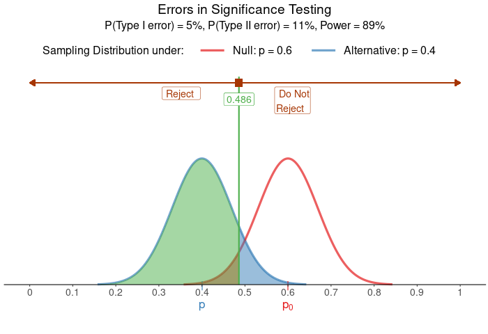

Power and Error relationship

Picture from Applet: https://istats.shinyapps.io/power/

9.3 Population Proportion Difference Test

Conditions

Check conditions for both $p_1$ and $p_2$

1. Random - Random Sample
2. Independence (10% Condition) - $n \leq 0.1N$
3. Normality (Large Counts) - $np_0 \geq 10, \space n(1-p_0) \geq 10$

Combined proportion

Assuming $p_1 = p_2$,

\[\hat p_C = \frac{X_1 + X_2}{n_1 + n_2}\]

When we assume $p_1 = p_2$, we are thinking that there was no difference in two samples. So, we are thinking like we got one larger sample with the size of $n_1 + n_2$.

This also decreases the variability of sampling distribution of proportion since we are increasing the sample size, and it would likely be closer to the true proportion if null hypothesis of $p_1 = p_2$ is true.

Standardized test Statistic

\[\begin{gather} z_{\hat p_1 - \hat p_2} = \frac{(\hat p_1 - \hat p_2) - (p_1 - p_2)}{\sqrt{\frac{\hat p_C (1- \hat p_C)}{n_1} + \frac{\hat p_C(1- \hat p_C)}{n_2}}} \end{gather}\]

Since we are assuming that $p_1 = p_2$, the equation can be simplified like below.

\[\begin{gather} z_{\hat p_1 - \hat p_2} = \frac{\hat p_1 - \hat p_2}{\sqrt{\frac{\hat p_C (1- \hat p_C)}{n_1} + \frac{\hat p_C(1- \hat p_C)}{n_2}}} \end{gather}\]